Time and Frequency Analysis Methods on GW Signals
Background Notes by X. Li
Part I: Basic Transform Methods
1.1 Revisit Continuous Fourier Transform and Discrete Fourier Transform
Continuous Fourier Transform:
Discrete Fourier Transform:
where we let
and
1.2 Chirp Z Transform
The chirp Z-transform (CZT) is a generalization of the discrete Fourier transform (DFT). While the DFT samples the Z plane at uniformly-spaced points along the unit circle, the chirp Z-transform samples along spiral arcs in the Z-plane, corresponding to straight lines in the S plane.[1][2] The DFT, real DFT, and zoom DFT can be calculated as special cases of the CZT. ( - Wikipedia)
To obtain DCZT from DFT, we introduce
where
thus, the DFT becomes
where a complex chirp is introduced via
Discrete Chirp Z Transform (*to be verified):
Compute with FFT & IFFT:
Some notes:
When computing using FFT, the signal in the block is treated as periodic**(to be verified), however, the input signal itself does not need to be.
Fresnel integral approximation?
1.3 Gabor Transform
The Gabor transform is a special case of the short-time Fourier transform. It is used to determine the sinusoidal frequency and phase content of local sections of a signal as it changes over time. The function to be transformed is first multiplied by a Gaussian function, which can be regarded as a window function, and the resulting function is then transformed with a Fourier transform to derive the time-frequency analysis. ( - Wikipedia)
Continuous Gabor Transform:
where the window function is a Gaussian in the form of
the width of which can be controlled via a scaling parameter α.
Thus the scaled Gabor is
Inverse Gabor Transform:
Gabor Expansion:
Discrete Gabor Transform (*to be verified):
1.4 S Transform
The S transform is a generalization of the short-time Fourier transform (STFT), extending the continuous wavelet transform and overcoming some of its disadvantages. Modulation sinusoids are fixed with respect to the time axis; this localizes the scalable Gaussian window dilations and translations in S transform. The S transform doesn't have a cross-term problem and yields a better signal clarity than Gabor transform. ( - Wikipedia)
Continuous S Transform:
where
Inverse S Transform:
Spectral Form:
where X(t) represents the Fourier Transform. (Convolution is used to get this spectral form)
Let
We obtain the
Discrete S Transform:
Implementation:
x Step1.Compute {\displaystyle X[p\Delta _{F}]\,} X[p\Delta _{{F}}]\, loop{ Step2.Compute {\displaystyle e^{-\pi {\frac {p^{2}}{m^{2}}}}} e^{{-\pi {\frac {p^{2}}{m^{2}}}}}for {\displaystyle f=m\Delta _{F}} f=m\Delta _{{F}} Step3.Move {\displaystyle X[p\Delta _{F}]} X[p\Delta _{{F}}]to {\displaystyle X[(p+m)\Delta _{F}]} X[(p+m)\Delta _{{F}}] Step4.Multiply Step2 and Step3 {\displaystyle B[m,p]=X[(p+m)\Delta _{F}]\cdot e^{-\pi {\frac {p^{2}}{m^{2}}}}} B[m,p]=X[(p+m)\Delta _{{F}}]\cdot e^{{-\pi {\frac {p^{2}}{m^{2}}}}} Step5.IDFT( {\displaystyle B[m,p]} B[m,p]). Repeat.}1.5 Constant Q Transform
CQT transforms a data series to the frequency domain. It is related to the Fourier transform[1] and very closely related to the complex Morlet wavelet transform.[2]
The transform can be thought of as a series of filters f**k, logarithmically spaced in frequency, with the k-th filter having a spectral width δf**k equal to a multiple of the previous filter's width:

where δf**k is the bandwidth of the k-th filter, fmin is the central frequency of the lowest filter, and n is the number of filters per octave. ( - Wikipedia)
Shifted (m) STFT:
given data with sampling frequency fs = 1/T, we have filter width δf_k and quality factor Q such that
Our window length of the k_th bin is therefore
making the relative power for each bin decrease at higher frequencies. To compensate this effect, we normalize the bin length by itself N[k].
Using the Hamming Window as an example, the normalization is
with
Finally, the Discrete Constant Q Transform:
Notes:
CQT is well suited to music data as the out put of the transform is effectively amplitude/phase against log frequency which is useful when the frequency spans several octaves. However, in the case of gravitational waves
1.6 Implementation on Chirp Signal (Windowed FFT - Tukey window)
In [1]:
xxxxxxxxxximport numpy as npimport matplotlib.pyplot as pltIn [2]:
xxxxxxxxxxdt = 0.001t = np.arange(0,3,dt)f0 = 50f1 = 250t1 = 2x = np.cos(2*np.pi*t*(f0 + (f1 - f0)*np.power(t, 2)/(3*t1**2)))fs = 1/dt#Chirp signalplt.plot(t, x)
In [3]:
xxxxxxxxxxfrom scipy import signalIn [4]:
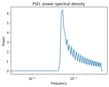
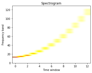
xxxxxxxxxxfreqs, times, spectrogram = signal.spectrogram(x)#Scipy PSD Power Spectral Densityfreqs, psd = signal.welch(x)plt.figure(figsize=(5, 4))plt.semilogx(freqs, psd)plt.title('PSD: power spectral density')plt.xlabel('Frequency')plt.ylabel('Power')plt.tight_layout()#Scipy Spectrogramfreqs, times, spectrogram = signal.spectrogram(x)plt.figure(figsize=(5, 4))plt.imshow(spectrogram, aspect='auto', cmap='hot_r', origin='lower')plt.title('Spectrogram')plt.ylabel('Frequency band')plt.xlabel('Time window')plt.tight_layout()
1.7 On the implementation of Time-Frequency Analysis for CNN
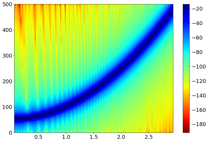
Constant Q Transform's high resolution at low frequencies is desirable in many cases for accurate analysis of the signal in both the time and frequency domain. However, when applying CQT for the purpose of identifying specific features on a spectrogram, high resolution in certain directions also means less obvious feature representation in certain cases (this assumption is highly dependent on the type of data you have). The Q range also affects the result significantly.
Some examples on GW chirp signal:
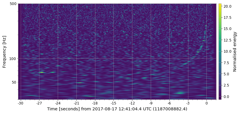
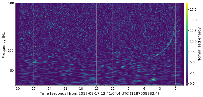
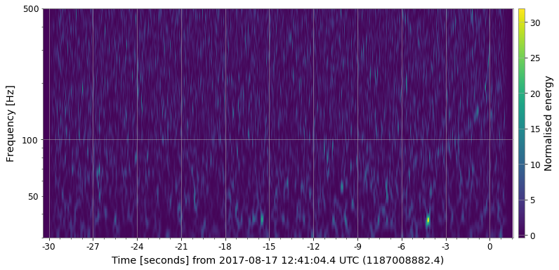
Thus, the time and frequency sampling width/length need to be adjusted accordingly for performance and resolution.
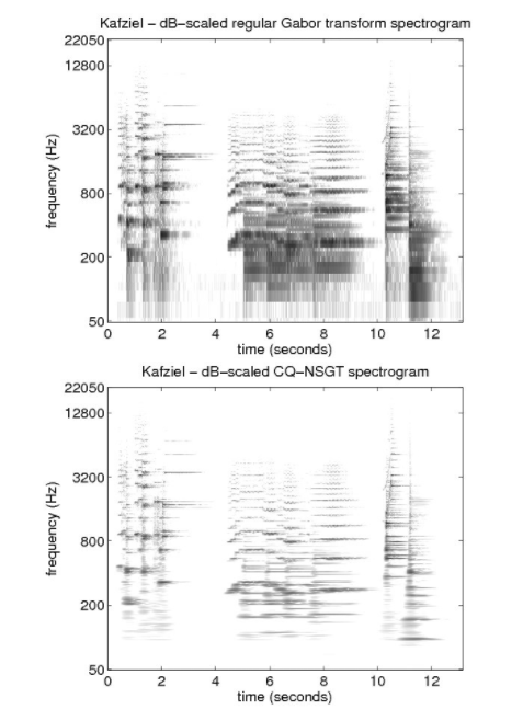
A spectrogram can also be inverse transformed to time-domain. Taking the generated chirp signal as an example:
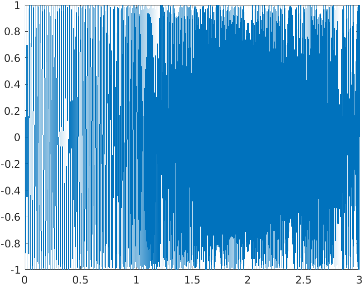
is the original chirp signal.
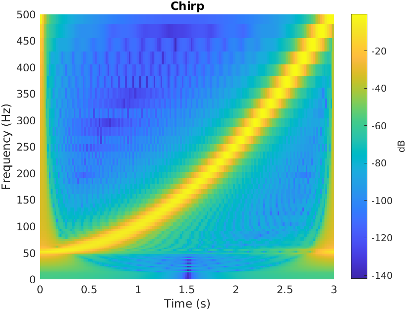
is the spectrogram using invertible Constant Q - Nonstationary Gabor Transform (Matlab CQT).

is the inverse transformed chirp signal.
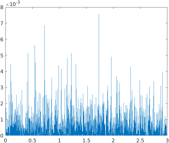
is the magnitude difference between the original chirp signal and the inverse transformed chirp signal.
1.8 Resources on CQT
Invertible CQT: https://www.univie.ac.at/nonstatgab/cqt/index.php (Useful for the Spectrogram Denoising and Time-series parameter estimation)
Gabor Wavelets (bob package): https://pythonhosted.org/bob.ip.gabor/guide.html#gabor-wavelets
Window Functions (Wikipedia): https://en.wikipedia.org/wiki/Window_function
On the discrete Gabor transform and the discrete Zak transform: http://www.martinbastiaans.org/pdfs/sigpro.pdf
Part II: Transform Methods Targeting Chirp Signals
2.1 Fractional Fourier Transform (FrFT)
The Fractional Fourier Transform is a family of linear transforms generalizing the Fourier Transform. It can be thought of as the Fourier Transform to the n-th power, where n need not be an integer. Thus it can transform a function to any intermediate domain between time and frequency. Its applications range from filter design and signal analysis to phase retrieval and pattern recognition.
A completely different meaning for fractional Fourier Transform was introduced by Bailey and Swartztrauber as essentially another name for a z transform, and in particular for the case that corresponds to a discrete Fourier transform shifted by a fractional amount in frequency space (multiplying the input by a linear chirp) and evaluating at a fractional set of frequency points. ( - Wikipedia)
The FrFT provides a continuous representation of a signal from the time to the frequency domain at intermediate domains by means of the fractional order of the transform that changes from -pi/2 to pi/2. (- The DLCT and its Applications 2013)
Continuous Fractional Fourier Transform
where alpha is the fractional order and K_alpha(t,u) is the kernel of the transformation which is defined as
When alpha = 0, the FrFT of the signal x(t) is the signal itself, while if alpha = -+pi/2, the FrFT becomes the Fourier Transform.
Inverse Continuous Fractional Fourier Transform
where * stands for the complex conjugate.
Discrete Fractional Fourier Transform
where the Kernel of the transformation has the following spectral expression
where nu_k(n) is the kth discrete Hermite - Gaussian function and M = {0, ..., N-2, N-N mod2}.
Inverse Discrete Fractional Fourier Transform
For a discrete signal x(n), we can define the connection between the fractional order (\alpha) and the chirp rate (\gamma) as
More info see The DLCT and its Applications 2013
2.2 Discrete Chirp-Fourier Transform
Discrete Chirp-Fourier Transform
where k represents the frequencies and r is an arbitrarily fixed integer that represents the chirp rates. The DCFT is the same as the DFT when r = 0. (page 5)
Inverse Discrete Chirp-Fourier Transform
The DCFT approximates the chirp rate by integer numbers r. Therefore, when using the DCFT to detect a chirp signal, the discrete chirp rate r0 of the signal should be an integer to guarantee that the parameter can be matched and that the peak will not be lost. This restriction affects the practical applications of the DCFT. (page 5)
More info see The DCFT and its Applications 2013
2.3 Linear Chirp Transform
The DLCT uses discrete complex linear chirp bases. It is not a time-frequency but rather a frequency chirp-rate transformation, implementable using Fast Fourier Transform. The Discrete Fourier Transform is a special case of the DLCT which has the properties of modulation and duality in time and frequency. (page 6)
Continuous Linear Chirp Transform
(Other conditions see DCFT and its Applications 2013)
Inverse Continuous Linear Chirp Transform
The CLCT can provide us with the same bandwidth of sinusoid signals if we intent to filter linear chirps in the frequency chirp-rate space. Thus, the CLCT can eliminate the effect of the chirp rate on the channel bandwidth of chirp communication systems (page 11, more in chapter 6) if we filter the signal at the corresponding chirp rate.
Discrete Linear Chirp Transform
Inverse Discrete Linear Chirp Transform
Note: One could think of the DLCT as a generalization of the DFT
If m = 0, then X(k,0) is the DFT of x(n) or the representation using chirp base with zero chirp rates. (page 15)
Properties of the Discrete Linear Chirp Transform (page 17):
Properties of the DLCT are similar to those of the DFT.
- Modulation property...
- Duality property...
Implementation with the FFT (page 19)
The DLCT can be implemented using the FFT. Rewriting X(k,m) as
and let
then for each -L/2 ⩽ m0 ⩽ L/2 - 1 the X(k, m0) is the DFT of h(n,m0) which can be obtained by the FFT.
The IDLCT can be implemented using the inverse FFT. Rewriting the expression for x(n) as
and let
where g(n,m) is the inverse DFT for each -L/2 ⩽ m0 ⩽ L/2 - 1. Then
If a vector X = [x(0)...x(N-1)]^T then
or the diagonal of the product of an N×L matrix.
G = {g(n, m)} with an L × N matrix E = {e(m, n) = exp(j2πCmn2/N )}
2.4 Cosine Chirp Transform
Page 22
Discrete Cosine Chirp Transform
a generalization of the Discrete Cosine Transform and X(k,0) is equal to the DCT of x(n).
The DCCT decomposes a signal using real linear chirps as
Inverse Discrete Cosine Chirp Transform
FFT Implementation
page 25
Forward:
where
Inverse:
where
Comments
The DCCT is a linear transformation - the signal x(n) = alpha x1(n)+ beta x2(n) has the DCCT X(k,m) = alpha X1(k,m) + beta X2(k,m)
Part III: Characteristics
3.1 Compare DLCT with FrFT
The DLCT just like the FrFT can be used to convert non-sparse signals into sparse signals in time or frequency. (page 27)
Sparsity
Sparsity or compressibility reflects the fact that information carried by certain signal is much smaller than their bandwidth. Most signals are not sparse in the time domain, so linear transformation are used to make the sparse in either time or frequency using certain basis. Stationary signals, such as sinusoids or quasi-periodic speech segments, are well represented by the Discrete Cosine Transform. The DCT can be used to obtain a sparse representation in frequency for such signals. However, non-stationary signals, such as chirps may not be sparse in either time or frequency, but rather in an intermediate domain. (page 27)
Resolution
A critical point of the time-frequency analysis and signal separation is the resolution of the transform. The DLCT and the DFrFT have been used to separate linear chirps in the time-frequency plane by projecting them and then followed by a filtering or a windowing procedure. If the resolution of the transform is good, even very close harmonics can be separated easily and vice versa. (details see page 31)
Peak Location
All the algorithms that use the DLCT or the DFrFT for parametric characterization of chirps depend on searching for peaks for all possible chirp rates or fractional orders to obtain the optimal chirp rate or the optimal fractional order that maximizes the |DLCT{x(n)}| or equivalently |DFrFT{x(n)}|. Therefore, it is obvious that the peaks should occur at the corresponding chirp rates and frequencies. (page 32, + example)
3.2 Estimation of Linear Chirp Parameters
Kalman Filtering is used to estimate parameters of chirps in -
[35] W. El Kaakour, M. Guglielmi, J. M. Piasco, and Le Carpentier, “Two identification methods of chirp parameters using state space models,” in Proc. of IEEE International Conference on Digital Signal Processing, Greece, vol. 2, Jul. 1997, pp. 903-906.
[36] M. Adjrad, A. Belouchrani, and A. Ouldali, “Estimation of chirp signal parameters using state space modelization by incorporating spatial information,” in Proc. of IEEE Seventh International Symposium on Signal Processing and Its Applications, France, vol. 2, Jul. 2003, pp. 531-534.
... (page 34)
Chirplet Decomposition
3.3 Sparsity and Compression
Sparsity in frequency is a key characteristic we are looking for. (High SNR, High CR, examples page 40)
Part IV: Types of Chirp Signals and GW Signal Compression
Linear Chirp
A linear chirp is a function whose frequency changes linearly with time. For example, a linear chirp has an instantaneous frequency
at time t. This is one of the reasons we need to use linear chirp bases instead of the classical Fourier bases because they are more suitable for representing the frequency changes of non-stationary signals. (page 10)
Quadratic Chirp
Logarithmic Chirp
Part V: Decomposition of Non-stationary Signals
5.1 Empirical Mode Decomposition
The Hilbert-Huang transform method was developed to represent non-stationary signals in the time-frequency plane without assistance of window functions. It is a combined approach of Hilbert transformation and the empirical mode decomposition. The EMD is used to decompose the signal into a set of functions called Intrinsic Mode Functions (IMFs). It does not have priori defined basis function, unlike the Fourier and Wavelet transform, the whole decomposition is adaptive and depends on the local oscillation of the data.
The decomposition is based on the local characteristics time scale of the data and, therefore, it is applicable to nonlinear and non-stationary processes.
Hilbert Transform is applied to each intrinsic mode function for the purpose of providing the global time-frequency distribution of the underlying signal to estimate its instantaneous frequency. The application of the HHT method to audio and speech signals have already been done. (The HHT is used to estimate the IF of biomedical signals)
5.2 Instantaneous Frequency Estimation
The Hilbert Transform is used to compute the IF of each of the signal components. (page 53)
Compare IF estimation results of DLCT and EMD. (page 54)
The performance of the EMD as an IF estimator is very much affected by the presence of the noise. Comparing the estimated IDs based on the DLCT and the EMD of both experiments with the actual IFs, we conclude the DLCT decomposition attains better results than EMD.
5.3 Time-Frequency Analysis using DLCT
Time-frequency distributions (TFDs) are frequently used for IF estimation based on peak detection techniques. The most frequently TFD used for linear chirps is the Wigner-Ville distribution (WVD) due to its ideal representation for such signals. However, in the case of multi-component signals, Wigner-Ville distribution does not perform well because of the presence of extraneous cross-terms. (page 56)
An algorithm that combines the DLCT with the Wigner-Ville distribution to obtain a time-frequency representation with high resolution.
Locally the DLCT approximates the signal as a sum of linear chirps, for each of which the WVD provides optimal representations. Superposing these WVDs we obtain a time-frequency representation of the whole signal without interfering cross-terms. (page 57)